Getting started with well log data

Last year, I wrote a post on DLIS files, one of the most common file formats for well log data. In it, I covered a few different approaches to extract data from such files. It seems like many people struggle with this, because that post quickly became my most popular one. Well over a thousand views later, it’s time to follow it up.

I have been working with acoustic well log data since 2018. During that time, I have learned a lot about how to work with such data, and I have been wanting to share my knowledge. To do so, I teamed up with Equinor’s Erlend Hårstad and Jørgen Kvalsvik, developers of the dlisio library. Since January, we have been working on a tutorial on how to use dlisio to work with well log data. As I am an acoustician, the tutorial naturally focuses on acoustic tools. However, much of what we show is general, valid for data from any tool.

We first presented this work at the 43rd Scandinavian Symposium on Physical Acoustics in the end of January. Just last week, we published the article that we wrote for the symposium’s proceedings. Along with it, we published a companion Jupyter Notebook, which contains the code underlying the article and some further details. As of June 2020, you can even run it on Binder, so that you can play with it online without having to download anything.

Three issues with well log data

Let’s say that you are an academic researcher who wants to research well logging or to teach it to students. You could certainly work with theory or with computer simulations, but if you want to work with real-world data, three issues stand in your way:

1. Getting data is hard. Well log data is typically owned by oil and gas companies. They consider their data sensitive, and do not release it easily.
2. If you get log data, chances are good that you’ll get DLIS files. As I covered in my previous blog post, this is a notoriously tricky format to deal with. And between the format’s standardisation in 1991 and 2018, no free software to programmatically extract data from DLIS files existed.
3. After you’ve extracted the data, you will probably not really know what the different pieces of data you’re looking at represent. A DLIS file contains fairly minimal documentation of its contents, and publicly available documentation on tools’ data is typically scarce.

Overcoming the issues

In the article, we explain how to overcome these issues. First, after Equinor released their open Volve Data Village dataset in 2018, getting data is not as hard. Among many other things, it contains 16.3 GB of various types of well log data. (Still, there is of course no guarantee that it has the exact type of data that you are looking for.)

The second issue is today more or less solved by the dlisio Python library. This is a free and open-source Python library to programmatically read data from DLIS files. While the library was fairly barebones when it was first released in 2018, its developers have been constantly improving it. Today, there’s not much in a DLIS file that dlisio can’t give you. While reading DLIS files is never going to be totally straightforward due to the awkwardness of the format, dlisio makes it about as easy as it can be. To help you along, our article covers the basics of what you need to know about DLIS files to effectively deal with them.

The third issue, however, is still very much present. However, we show in the article how you can use dlisio to investigate and understand scarcely documented tool data. While the article focuses on sonic and ultrasonic tools used in the Volve integrity logs, you can take a similar approach for other tools’ data.

Investigating well log data

In the article, we dig into one particular integrity log from the Volve dataset. We investigate the sonic and ultrasonic data therein, and give an idea of what you can do with it. While you will have to read the article or peruse the notebook to get the full picture, I’ll give you a quick overview of what they cover.

Sonic data

The sonic data in the file was recorded by Schlumberger’s Digital Sonic Logging Tool (DSLT). This is a fairly standard cement bond log tool with one transmitter and two receivers 3 and 5 ft away. Putting it very briefly, the transmitter shoots sonic pulses, and the receivers record the resulting waveforms. The start of a waveform may look something like this:

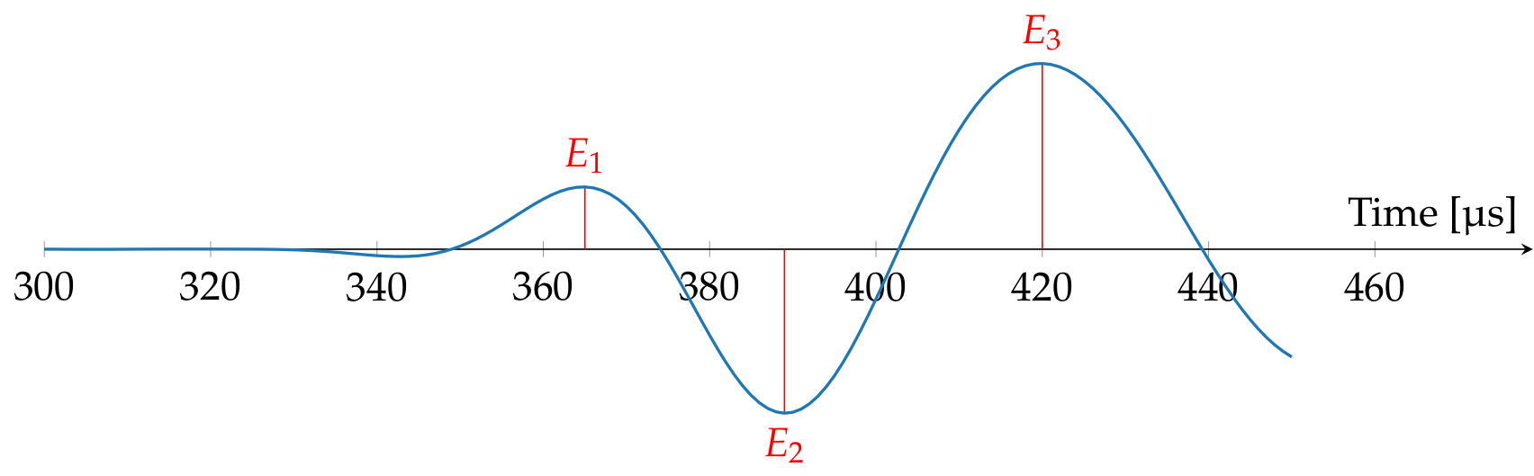
This first component of the waveform has travelled along the casing, the fastest path from the transmitter to the receivers. The main feature drawn from the waveforms is the first peak amplitude \(E_1\). This is also known as the cement bond log (or CBL), and can give you a general idea of whether solids are bonded to the outside of the casing.

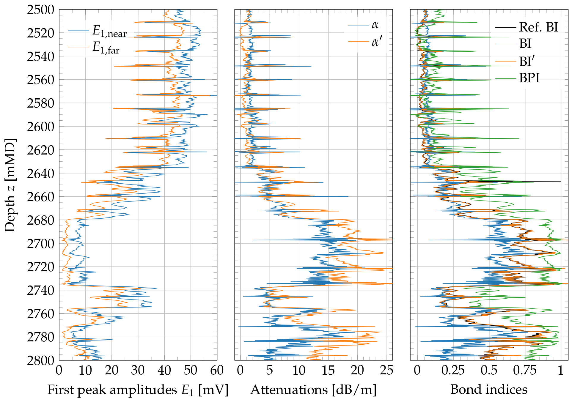
The sonic data in the file contains waveforms for the near and far receivers, measured every 2 inches along the well. It also contains various data derived from the waveforms, such as CBL amplitudes, transit times, and a bond index. In the article and notebook, we go into how you can calculate those derived quantities, and other quantities not provided in the file, from the waveforms.

Ultrasonic data

The ultrasonic data was recorded by Schlumberger’s Ultrasonic Imaging tool (USIT). This tool has a rotating transducer that fires ultrasonic pulses. Depending on the desired resolution, it can probe the well every 5° or 10° at every depth. The transducer records the waveforms reflected from the casing. At a particular depth, the waveforms might look like this:

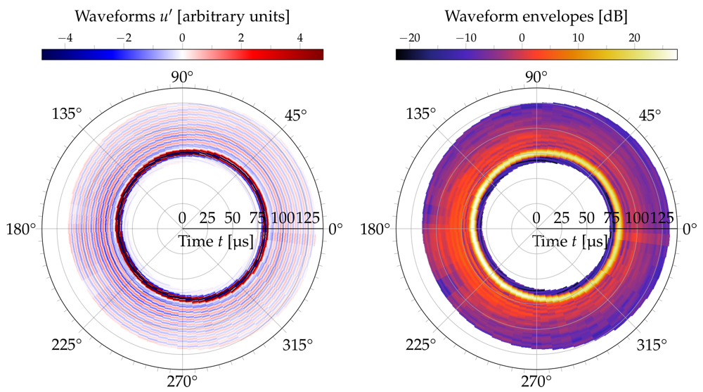
Such waveforms can then be processed to estimate various types of information: The tool’s eccentering, the casing’s inner radius and thickness, and the impedance of the material behind the casing. The well log data file already contains the results of such a processing. However, it’s also possible to reprocess the data yourself, perhaps using a different method.

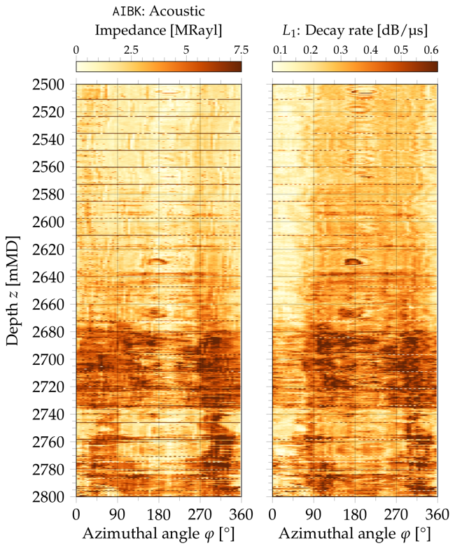
As a simple example of such reprocessing, we calculated the decay rate used by Sirevaag et al. to analyse their own measurements. This estimates how fast the resonant tail of the envelope decays. Fast decays indicate solids behind the casing, while slow decays indicate fluids.

The plots to the right show a comparison between the acoustic impedance stored in the file and the reprocessing we performed. While the reprocessing is more affected by eccentering and third interface echoes, the overall picture is the same. This shows how we can use well log data to test and compare different types of processing on real-world cases.

What you can do next

If you want to read data from DLIS files, you can first have a look at our article, especially the first two sections. Taking a quick look at Sections 3 and 4 may also be a good idea, as they give you pointers on figuring out how the tools you are interested in store their data. You can then use the notebook as a jumping-off point for your own work. The notebook shows various best-practice examples of how to use dlisio to read data from DLIS files. It also contains a number of handy functions for inspecting and plotting data.

If you’re particularly interested in acoustic data, then you may want to take a closer look at Section 3 of the article, as well as the notebook. Through them, you can learn the basics of how the DSLT and USIT tools store their data. Even if you want to work on different acoustic tools, there may be some similarities to the DSLT and the USIT that you can exploit. And if you’re planning on doing something interesting with acoustic data, I’d love to know! You can send me a tweet, an email, or simply comment on this post.