Acoustic quantities, part 3: Time variation

In this series, we first looked at what sound pressure levels and decibels are. Then, we looked at how we can calculate sound pressure levels in a way that takes human hearing into account. So far, though, we have only considered steady and unchanging sounds. These come from e.g. ventilation systems or machines that run steadily. But what about sounds that change in time, e.g. sounds from passing cars or aircraft, or from explosions and other bangs? Fortunately, acoustic quantities and techniques exist that allow us to describe and compare these sounds as well. The most important are Slow- and Fast-weighting, sound exposure level, and equivalent level. These are the topics of this part of the series.

Weighting, Fast and Slow

In the first part, we saw how we can compute a sound pressure level from the RMS pressure, which is a kind of representative sound pressure. To find the RMS pressure, we first measure the sound pressure of a steady sound over a long enough period. Then, we boil it down to a representative number for that sound. But what if we want to characterise a sound that is not steady? In that case, we can determine a sound pressure level that changes with time: How strong is the sound now? How strong was it a second ago? Or a minute ago?

Therefore, there exist several ways to weight sound in time. Thus, you can calculate the current sound pressure level for where you are based on the sound of the last few moments. A few different time weightings are in use. The most common have the delightfully simple and descriptive names Slow and Fast, and are constructed in the same way.

Exponential time weighting

More concretely, we apply this time weighting using the exponential functions in the figure to the right. These go towards zero as we go further back in time. What separates Slow and Fast is how quickly they go to zero. Fast has a “time constant” of 0.125 seconds. As you can see in the figure, it basically ignores anything that happened more than half a second ago. The time constant of Slow is eight times longer, at 1 second. This means that it “looks” eight times further back in time.

So, how do we use these time weighting functions? As when we calculate the RMS pressure, we start with the squared sound pressure, \(p^2(t)\). Now, however, we apply a time weighting function instead of calculating a simple average. We can express this mathematically as

\( p_T(t) = \sqrt{\frac{1}{T}\int_0^t p^2(\tau) \mathrm{e}^{-(t-\tau)/T} \, \mathrm{d}\tau} \, ,\)

where \(t\) is the time at which we are calculating the sound pressure level, and \(T\) is the time constant of Slow or Fast. Depending on which one we choose, we get the Slow-weighted sound pressure \(p_\mathrm{S}(t)\) or the Fast-weighted sound pressure \(p_\mathrm{F}(t)\). In turn, we can use these to calculate the Slow- or Fast-weighted sound pressure levels,

\(L_\mathrm{S}(t) = 20 \log \left( \frac{p_\mathrm{S}(t)}{p_\mathrm{ref}} \right) , \qquad L_\mathrm{F}(t) = 20 \log \left( \frac{p_\mathrm{F}(t)}{p_\mathrm{ref}} \right) .\)

These formulas are wisely designed such that they give the same sound pressure levels as the simple RMS procedure for steady sounds.

Examples

To make things more clear, let us look at the examples of Slow and Fast weighting below. In both examples, we use a two-second burst of pink noise, starting at \(t=0\). (We assume complete silence before then.) You can see this noise in the subfigures to the left. The middle subfigures show how we weight the squared sound pressure when we calculate the Slow- and Fast-weighted sound pressure for \(t=2\). The subfigures to the right compare the time-varying Slow and Fast sound pressures with the RMS sound pressure \(p_\mathrm{RMS}\).

Slow

Fast

In both cases, we see that the Slow- and Fast-weighted sound sound pressures correspond to the RMS sound pressure in the end. Because Fast does not look as far back in time and therefore reacts more quickly, it approaches the RMS sound pressure faster. At the same time, we see that Fast wobbles a bit. Since it does not look as far back, it is more susceptible to short-term random changes in the noise. (No noise is perfectly steady!)

Note that these examples show Slow- and Fast-weighted sound pressures in Pascal, and not sound pressure levels in decibels. To find the sound pressure level from the sound pressure, we must use the above formula.

Summary

Slow and Fast time weighting both give sound pressure levels based on what has happened in the last few moments. The two have somewhat different uses, though:

• Slow-weighted sound pressure levels \(L_\mathrm{S}\) look further back in time. This makes the levels change slowly and evenly, suppressing impulsive sounds and random sound variations. Slow is best used for sounds that vary slowly, such as the sound from passing aircraft.
• Fast-weighted sound pressure levels \(L_{F}\) do not look as far back in time. This makes the levels more uneven, but also lets us catch impulsive sounds. Fast is best for shorter sounds, such as explosions and other bangs. Just look at the figure to the right to see how much more Fast reacts to the sound of a starting pistol.
• For steady sounds where the loudness does not vary in time, Slow and Fast will both correspond to the sound pressure level based on RMS pressure.

Maximum level

Slow and Fast time weightings show us how the sound pressure level varies in time. However, we cannot easily characterise sound pressure levels with time-varying quantities. We would rather have one number describing how loud the sound is.

The simplest way to find such a number is to just find the highest value in the curve for Slow- or Fast-weighted sound pressure or sound pressure level. This gives us an indication of how loud the sound is at its loudest. The figure to the right shows how we find Fast-weighted maximum sound pressure. We can then calculate the maximum sound pressure level from this as

\(L_\mathrm{Fmax} = 20 \log \left( \frac{p_\mathrm{Fmax}}{p_\mathrm{ref}} \right) .\)

If we already have curves of the Slow- or Fast-weighted sound pressure levels, we can also find the maximum level directly from these. The result is the same.

Noise dose: Sound exposure level

One weakness of maximum levels is that they only describe how loud the sound is at its strongest. They say nothing about how long the sound lasts. For example, we might find the same maximum level from a helicopter flying over you and a helicopter hovering above you for an hour, but the latter event is obviously more annoying.

The sound exposure level (or SEL) gives us a number in decibels for how much sound we have been exposed to in total over a period of time. It thus represents a kind of noise dose. This time period can be long, such as a concert or a workday, or it can be as short as a single sound event, for example one aircraft pass-by.

The sound exposure level is calculated almost in the same way as the RMS pressure, explained in the first part of this series, with one difference. When we compute the RMS pressure, we integrate the squared sound pressure \(p^2(t)\) over a time interval and divide by the length of the interval to get the averaged squared sound pressure. When we calculate the sound exposure pressure, however, we divide by a reference time of one second:

\( p_\mathrm{E} = \sqrt{\frac{1}{\text{1 second}} \int_{T_1}^{T_2} p^2(t) \, \mathrm{d}t} \, .\)

Then, we calculate the sound exposure level from this sound exposure pressure:

\(L_\mathrm{E} = 20 \log \left( \frac{p_\mathrm{E}}{p_\mathrm{ref}} \right) \, .\)

Example

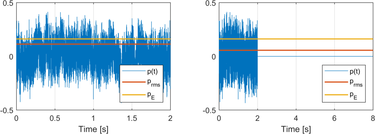
Let’s look at the sound exposure pressure and the RMS sound pressure for two cases:

• In the first case, we have a two second long clip of pink noise.
• In the second case, we have the same clip, followed by six seconds of silence.

Let’s compare the two cases in the figures below. We see that the RMS pressure is lower in the second case, while the sound exposure pressure is the same in both. The reason why the RMS pressure decreases is that the following silence makes the sound less loud on average. The sound exposure pressure, on the other hand, is the same in both cases. This is because we calculate it from the total amount of sound in the measurement period.

What, then, does the sound exposure level tell us? It is, after all, somewhat abstract and difficult to compare directly with the usual RMS sound pressure level. However, we can compare different sound exposure levels with each other. For example, take two workers that wear noise dosimeters throughout their workday. After the day is done, we can compare their sound exposure levels to see who was exposed to the most noise.

Equivalent level

Like the sound exposure level, the equivalent level resembles the RMS sound pressure level. The only difference between this and the sound exposure level is that we spread the sound exposure over a longer period \(T\) instead of just one second. Thus, we calculate the equivalent pressure and level as:

\( p_{\mathrm{eq},T} = \sqrt{ \frac{1}{T} \int_{T_1}^{T_2} p^2(t) \, \mathrm{d}t } \, , \qquad p_{\mathrm{eq},T} = 20 \log \left( \frac{p_{\mathrm{eq},T}}{p_\mathrm{ref}} \right) \)

The equivalent level thus takes the sound exposure from a time period and spreads it over the same (or another) time period.

Example

For example, we can take all the noise that you were exposed to yesterday, and spread it over 24 hours. This gives us the 24-hour equivalent level \(L_{\mathrm{eq,24h}}\), but what does it tell us? Well, this equivalent level represents the sound pressure level of a steady sound that would give the same noise dose as all of the sound that the equivalent level is based on.

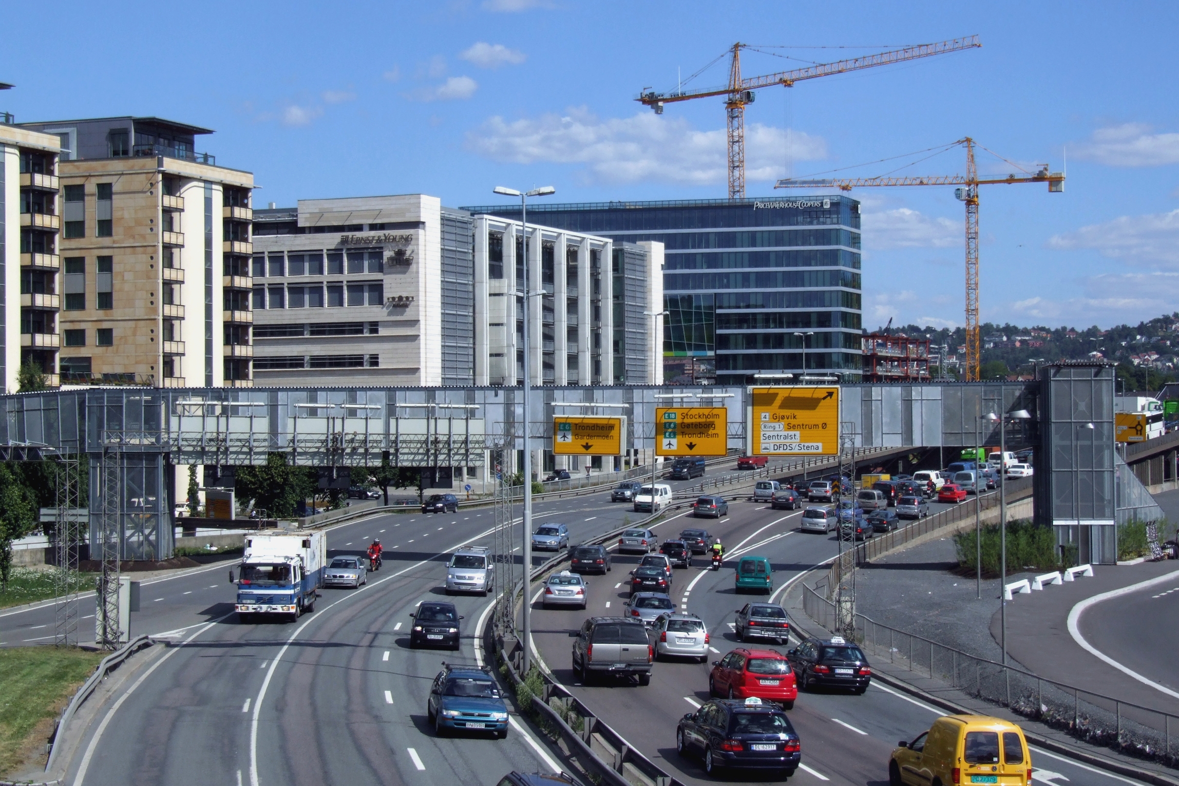
If the equivalent noise level is based on only one noise event, it becomes a somewhat abstract acoustic quantity similar to the the sound exposure level. On the other hand, if we calculate e.g. a one-hour equivalent level \(L_\mathrm{eq,1h}\) for rush hour traffic, we get a nice and representative quantity for the time-varying sound pressure level in that period. For that reason, noise regulations (at least in Norway) are mainly based around variants of equivalent levels. We will take a closer look at these in the next part.

In combination with frequency weighting

It is not difficult to combine time and frequency weightings. As we saw in the previous part, we perform frequency weighting by filtering the original sound pressure \(p(t)\) to get e.g. an A-weighted sound pressure \(p_\mathrm{A}(t)\). We can in turn take this frequency weighted sound pressure and time weight it in any one of the ways described above. For example, we can thus find e.g. sound pressure levels \(L_\mathrm{AF}(t)\), which have been A-weighted in frequency and Fast-weighted in time, or we can find A-weighted sound exposure levels \(L_\mathrm{AE}\). In practice, almost all public noise regulations incorporate a combination of A-weighting in frequency and some weighting in time.

Next time

In these three parts, we have explained the building blocks of the acoustic quantities used in noise regulations. However, these regulations use more advanced quantities that give a better picture of how annoying a noise situation is. (For more on the connection between noise and annoyance, you can read this blog post written by my friend and former colleague Femke Gelderblom.) In the next part, we will go through the more advanced quantities used in noise regulations in Norway and many other countries.

This post is a translation of a Norwegian-language blog post that I originally wrote for acousticsresearchcentre.no. I would like to thank Rolf Tore Randeberg for proofreading and fact-checking the Norwegian original.

Read the whole series on acoustic quantities

• Part 1: What are decibels?
• Part 2: Frequency weighting
• Part 3: Time variation
• Part 4: Quantities in noise regulations